The Finite Difference Method

Numerical simulations of physical processes generally involve solving some differential equation on a computational domain too complicated to solve analytically. Solving simple systems by “hand” is quite possible in one-dimension. But things get more complicated as you go to higher dimensions. If the domain has a nice shape – that is, if it’s rectangular or cylindrical in nature – you may be able to solve it analytically using techniques such as separation of variables. But as you start introducing irregularities in the boundary or in the forcing function, things start getting hairy really soon. In that case, going to a numerical solution is the only viable option.
The Finite Difference Method (FDM) is a way to solve differential equations numerically. It is not the only option, alternatives include the finite volume and finite element methods, and also various mesh-free approaches. However, FDM is very popular. The popularity of FDM stems from the fact it is very simple to both derive and implement numerically.


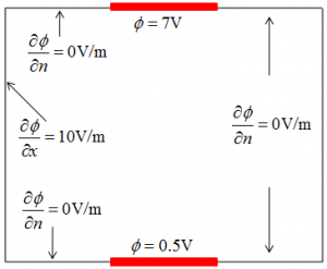
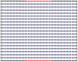
Figure 1. Problem definition (left) and domain discretization (right)
As an example, let’s consider the Poisson equation, \(\nabla^2\phi=-\dfrac{\rho}{\epsilon_0}\). This equations governs the variation of electric potential given some charge density distribution. It is one of the most fundamental equations in the field of electro-static plasma simulations. We want to solve this equation numerically on a rectangular domain shown in Figure 1 subject to the boundaries listed in the figure. The domain contains of two regions of fixed potential along upper and bottom edge – these could represent charged electrodes. Remaining edges have zero electric field, except for the left edge, on which electric field is specified.
We start by discretizing the domain – in other words, overlaying a computational mesh over the domain. In the Finite Difference method, solution to the system is known only on on the nodes of the computational mesh. As such, it is important to chose mesh spacing fine enough to resolve the details of interest. In addition, cell edges must coincide with the axis of the coordinate system being used. This is one of the main disadvantages of FDM: complex geometries cannot be directly resolved by fitting the mesh to the object boundary.
Finite Difference representation of derivatives
We are looking for the solution to \( \nabla^2\phi=\dfrac{\partial^2\phi}{\partial x^2}+\dfrac{\partial^2\phi}{\partial y^2}=-\dfrac{\rho}{\epsilon_0}\). From Taylor’s Series, we know that a value of a function some distance $latex \Delta x$ from a known point x can be estimated from derivatives as
$$ f(x+\Delta x)=f(x)+\dfrac{f'(x)}{1!}(\Delta x) + \dfrac{f”(x)}{2!}(\Delta x)^2 + \dfrac{f”'(x)}{3!}(\Delta x)^3+ O(4)+\ldots $$
In other words, the second derivative at x given by
$$f”(x) = \dfrac{2}{\Delta^2x}\left[ f(x+\Delta x) – f(x) – f'(x)\Delta x – \dfrac{f”'(x)}{6}\Delta^3 x+ O(4)+\ldots \right]$$
The expression above is known as the forward difference. We are estimating the derivative at a point using data to the front (in positive direction) of that point. We can obtain a similar expression by going backward
$$f(x-\Delta x)=f(x)+\dfrac{f'(x)}{1!}(-\Delta x) + \dfrac{f”(x)}{2!}(-\Delta x)^2 + \dfrac{f”'(x)}{3!}(-\Delta x)^3+ O(4)+\ldots $$
or
$$f”(x) = \dfrac{2}{\Delta^2x}\left[ f(x-\Delta x) – f(x) + f'(x)\Delta x + \dfrac{f”'(x)}{6}\Delta^3 x+ O(4)+\ldots \right]$$
We now have two expressions for the second derivative at point x. Instead of using one of the other, it’s best practice to use their average. By adding the two expression and dividing by two, we obtain the central difference representation for the second derivative:
$$f”(x) = \dfrac{f(x-\Delta x) – 2f(x) + f(x+\Delta x)}{\Delta^2x} + O(4) +\ldots$$
The first and third derivative conveniently cancel out, and the resulting expression is second-order accurate.
Numerical Implementation
On the computational domain, potential is no longer a continuous function, instead, it is given by a collection of values at node indices as phi[i][j]. Assuming uniform spacing between the grid nodes in each directions, the second derivative in the x direction is written as d2f_dx2 = (phi[i-1][j]-2*phi[i][j]+phi[i+1][j])/(dx*dx). Adding the expression for the y direction, we obtain the discretized version of the Poisson equation:
(phi[i-1][j]-2*phi[i][j]+phi[i+1][j])/(dx*dx) + (phi[i][j-1]-2*phi[i][j]+phi[i][j+1])/(dy*dy) = -rho[i][j]/eps0
That’s it, quite simple. The expression above gives us an expression that can be used to solve for potential everywhere inside the domain. But to complete the problem, we need to include the boundaries.
Boundary Conditions
Our problem has two types of boundary conditions: fixed potential along portions of top and bottom boundary, and fixed derivative (electric field) on the remaining nodes.
The first case is known as Dirichlet boundary condition. It is simple to implement. On each node along the boundary we have phi[i][j]=g[i][j]
The second condition is known as Neumann. On the left face, we have \(\nabla \phi \cdot (-i)=-E_0\) or \(\dfrac{\partial \phi}{\partial y}=E_0\). From the Taylor expansion, the first derivative is given by
$$f'(x)=\dfrac{f(x+\Delta x)-f(x)}{\Delta x} + O(2) + \ldots$$
This is the forward difference for the first derivative. Central difference can be derived using process analogous to above. However, since we do not have any data in the backward direction along the y=0 face, we are forced to use this less-accurate representation. This equation is implemented numerically as (phi[i+1][j]-phi[i][j])/dx = E0
Numerical implementation
This simple example implemented in a simple Java Finite Difference Solver. Give the program a try (I used Eclipse to write it) and let me know if you have any questions.

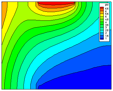
Figure 2. Solution to the sample problem using the Finite Difference Method.
For an alternative, see The Finite Volume Method.
Don’t forget to link to this article if you find it useful.
Please leave a comment if you have any questions. Thanks!
Hi,
I wonder how B[u]=1/(dx)^2, T[u]=1/(dy)^2 etc. were derived. I know it has something to do with the coefficient matrix but I cannot figure this out. For example, if the equation was again Poisson equation but the second derivative was multiplied by x^2, how do you compute these quantities?
Thanks in advance,
Dimitris
Ok, I figured it out. They are just the coefficients of the top, bottom, left, right and central node after you discretize the equation.
Great, and sorry for not getting back to you in time.
Have you considered making your java code an applet so that it can be embedded into the website?
Here is my web based javascript version of this solver.
http://dl.dropbox.com/u/5095342/PIC/solver.html
Wow, you rock! This is totally awesome. Here is a next task for you 🙂 Use VTK to extract isosurface from some 3D field, save as VRML, and show as 3D object.
Here is my 3D version of solver.
http://dl.dropbox.com/u/5095342/PIC/solver3D.html
I haven’t had the chance to look at VTK to find out what they do with isosurface. All I did was plot the computational mesh points calculated by solver in 3D.
Can you verify the neumann boundary conditions in your solver.java .
/* set neumann boundaries along the edges */
for (i = 0; i < nx; i++) {
/* bottom */
T[i] = 1 / dx;
C[i] = -1 / dx;
/* top */
B[(ny – 1) * nx + i] = 1 / dx;
C[(ny – 1) * nx + i] = -1 / dx;
}
Should the neumann boundary along the top and bottom be normal to the boundary. Does it make more sense to use 1 / dy instead of 1 / dx for the top and bottom boundary in the above equations. Also, are you supposed to perform a dot product with the (external) normal to the boundary, so does the top get multiplied by +1 (+y direction) and the bottom get multiplied -1 (-y direction) according to this wiki.
http://en.wikipedia.org/wiki/Neumann_boundary_condition
I came across this description for neumann boundary conditions math for a problem similar to the one in the article.
http://12000.org/my_courses/UC_davis/fall_2010/math_228a/HWs/HW3/Neumman_BC/Neumman_BC.htm#SECTION00030000000000000000
I came across this description for neumann boundary conditions math for a problem similar to the one in the article.
http://12000.org/my_courses/UC_davis/fall_2010/math_228a/HWs/HW3/Neumman_BC/Neumman_BC.htm
I tried using the math for Neumann Boundary conditions described in the above article and I get the following results.
http://dl.dropbox.com/u/5095342/PIC/solverNeumann.html
Does this look right to you?
In the original problem is says that the neumann boundaries on the top, bottom and right sides are dPhi / dn = 0 which indicates that they are insulated. In my output, the results I get are that these edges are colored blue and have low electric potential.
I think the equations in section 1.2 of the article dealing with insulated neumann boundaries du / dn = 0 is not quite right. I think the term in 1.2.2 for instance (hy / hx) * Uend-1,j should be added instead of subtracted. The same applies to the other insulated boundary equations in section 1.2 . Doing so gives a result that is similar to the one in this article. I also used the equations for the corner points from the boundary article for this latest result.
http://dl.dropbox.com/u/5095342/PIC/solverNeumann.html
I modified the solver routine to use a Full Multigrid Cycle to solve the problem. Here is the link to the solution using multigrid.
http://dl.dropbox.com/u/5095342/PIC/solverfmg.html
Here is an example of the Finite Difference Time Domain method in 1D which makes use of the leapfrog staggered grid.
http://dl.dropbox.com/u/5095342/PIC/fdtd.html
You can learn more about the fdtd method here.
http://en.wikipedia.org/wiki/Finite-difference_time-domain_method
and here.
http://www.eecs.wsu.edu/~schneidj/ufdtd/
Here is an example of the Finite Difference Time Domain method in 2D.
http://dl.dropbox.com/u/5095342/PIC/fdtd2d.html
Hello again! You have many interesting things on this site. I have two questions please: 1) Is the value -rho[i][j]/eps0 equal to zero for every cell? 2) And what value of dx did you use to get your nice colorful graph? I used dx = 0.01 because anything bigger Excel doesn’t like it (or it seemed so…). Thanks a lot for your generous time!!!
This depends on the local charge density. I believe it is zero in this particular example but in general it won’t be. Plasma is generally quasineutral, which means that rho is approximately zero at spatial scales greater than the Debye length. However, for a Poisson solver to converge, the cell size must be smaller or at least the order of the local Debye length, and at that spatial scale you will get some small deviations from quasineutrality. These deviations are the source of the restoring force that keeps ions and electrons close to each other.
About your second question, these plots were actually generated by Tecplot. Tecplot is a commercial program for data visualization. It is a very nice package, but it seems that every year it picks up more features you don’t need and the price goes correspondingly up. There are some free data visualization alternatives available, such as Paraview and VisIt. I have also developed my own visualization tool many years back called capVTE. Unfortunately, it does not currently work anymore, but I am hoping to revive it shortly.
I tried implementing this with Matlab over a square region with interval sizes the same in both directions. Here is an image of the result produced by Matlab.
http://dl.dropbox.com/u/5095342/PIC/fd_matlab.jpg
I based it on these video lectures of finite differences from MIT.
http://ocw.mit.edu/courses/mathematics/18-085-computational-science-and-engineering-i-fall-2008/video-lectures/lecture-2-differential-eqns-and-difference-eqns/
and
http://ocw.mit.edu/courses/mathematics/18-086-mathematical-methods-for-engineers-ii-spring-2006/video-lectures/lecture-12-matrices-in-difference-equations-1d-2d-3d/
I tweaked my matlab solution a little playing around with the boundary conditions. This is what matlab gives me when the left neumann boundary condition is 10. (First derivative in x direction set to 10)
http://dl.dropbox.com/u/5095342/PIC/johncoady/fd_matlab.jpg
And this is what I get when I set the left neumann boundary condition to -2 .
http://dl.dropbox.com/u/5095342/PIC/fdlb_2_matlab.jpg
I tried implementing this example using the Finite Element Method in 2D on MATLAB. This is the result that was produced.
http://dl.dropbox.com/u/5095342/images/fem2d.jpg
I based it on the FEM2D code described is this paper.
http://www.math.hu-berlin.de/~cc/download/public/software/documentation/acf.pdf
Finite Element MATLAB code can be found here.
http://people.sc.fsu.edu/~jburkardt/m_src/fem_50/fem_50.html
Here is another implementation using Finite Elements to solve in MATLAB and distmesh to generate the mesh.
http://dl.dropbox.com/u/5095342/images/fem2d2.jpg
I used distmesh to automatically generate a mesh of triangles.
http://persson.berkeley.edu/distmesh/
I also modified this MIT MATLAB code for a 2D Finite Element solver to read in the mesh data, add Neumann boundary conditions and solve the problem.
http://math.mit.edu/cse/codes/femcode.m
Here is one more example using 2D Finite Elements with distmesh on a disk shape object with boundary conditions of 0.5 and 7.0 on the inner and outer boundaries of the disk.
http://dl.dropbox.com/u/5095342/images/fem2d_disk.jpg
Hi, I know it’s been a while but I was wondering if you had any insight on having open boundary conditions. Something like PML for FDTD but for electrostatic problems? I can’t seem to find anything online.
As an example, if I want to model a square in the center of the simulation with an applied voltage? How would I go about having open boundary conditions?