Handling Surfaces: Line Triangle Intersection Example

In this article I will discuss my “favorite” topic: performing particle surface intersections. Here “favorite” is in quotes as I have spent embarrassingly too much time on this problem without still having a truly working solution. It’s also likely the reason my hair started falling out in grad school!
As your codes become more complex, you will eventually be interested in modeling plasma or gas flows around real-world objects that cannot be described with simple analytical shapes like cylinders or bricks. As we learned in PIC Fundamentals and Advanced PIC, there are two ways to handle the gas domain: structured and unstructured meshes. The structured (or Cartesian) mesh is more efficient when it comes to pushing particles and leads to a simpler formulation for the field solver. The downside is that your volume mesh boundaries will no longer line up with the geometry. We end up with two different meshes representing the problem: a Cartesian volume mesh that we use to compute field properties, and a surface mesh that is used to define particle boundaries. Here we ignore the topic of computing fields in the interface (or cut) cells and simply focus on the particle motion. The discussion is thus also relevant to free-molecular codes such as the Contamination Transport Simulation Program (CTSP).
Particle Loop Algorithm
Checking for surface intersections is conceptually simple. But as we will see, there are inherent challenges due to limited precision of computer floating point mathematics. The algorithm is as follows:
update particle velocities
for each particle:
    dt = system_dt
    while dt>0:
        x_old = x
        x = x + v*dt
        retrieve all surface elements in x_old:x box
        for each surface:
            check if ray (x_old:x) intersects element
            if yes, save if closer than previous closest hit

        if element hit:
            push particle to surface
            set bounce off velocity
            subtract fraction from dt used to reach the surface
        else:
            dt = 0
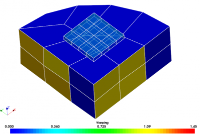
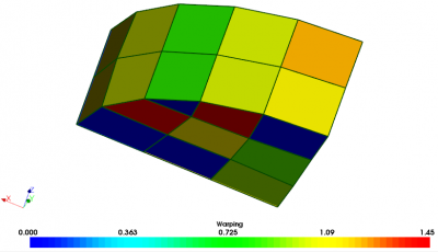
We will demonstrate this scheme with an example code that bounces particles inside a closed vessel described by a surface mesh loaded from a file. I used Salome to generate the model, shown in Figure 1 below. The main object consists of a section of a cylinder, in which the surface elements on the top face were collected into a “source” group. We will be injecting particles from these elements. The mesh was generated using the Netgen algorithm with quadrangles enabled. I purposely introduced anomalies to the model that you are likely to encounter in real world situation. Specifically, I manually shifted some of the nodes to introduce warp to the quadrangles. When I originally added support for quads to CTSP, I made the wrong assumption that quads are planar. This is not the case! While meshing tools attempt to minimize the amount of warp, it is not unreasonable to find quads warped 5 degrees or even more. Not taking warp into account will lead to particle leaks. I also added a small box sitting on top of the vessel. This box was introduced to add overlapping elements. As you will see, this overlap results in a leak.
Implementation
For brevity, I am going to skip going through most of the code, but basically its consists of 4 files: surf-int.cpp, surf-int.h, surface.cpp, and surface.h. The main code is defined in surf-int, while the surface files provide various structures and functions for storing the surface mesh and performing line-element intersections. I wanted to bring your attention to the particle loop, starting on line 154 in surf-int.cpp.
SurfaceElement *el_min = nullptr;
Particle &part = *it;

int bounces = 0;
const int max_bounces = 100;
double part_dt = dt0;
bool alive  = true;

/*particle loop*/
while(part_dt>0  && bounces++<max_bounces)
{
    double x_old[3];
    vec::copy(x_old,part.pos);

    vec::mult_and_add(part.pos,part.pos,part.vel,part_dt);

    //placeholder for retrieving elements from octree or a similar structure
    vector<SurfaceElement*> elements = surface.getElements(x_old,part.pos);

    /*intersect with surface triangles*/
    double t_min = 2;
    bool secondary_min = false;
    el_min=nullptr;

    for (SurfaceElement *el:elements)
    {
        //obtain parametric position of the intersection point
        double t = el->lineIntersect(x_old,part.pos,t_min);

        //check for intersection with secondary triangle on skewed quads
        bool secondary=false;
        if (t>=2.0) {t-=2.0;secondary=true;}

        //small positive offset to avoid self intersection with starting surfaces
        if (t<1e-8) continue;

        /*accept if closer than previous hit or if same but looking at us.*/
        if (t<t_min || (t==t_min && vec::dot(part.vel,el->normal)<vec::dot(part.vel,el_min->normal)))
        {
            t_min = t; el_min = el; secondary_min = secondary;
        }
    }

    /*if no particle impact*/
    if (el_min==nullptr)
    {
        part_dt=0;
    }
    /*we have impact!*/
    else
    {
        /* ... */
    }
}    /*dt loop*/
This is the code that pushes a single particle through multiple bounces. We start by advancing the particle position through the entire time step – think of this as the time interval through which the particle still needs to move to catch up to the current simulation time. We then somehow obtain the list of surface elements (triangles or quads) that need to be checked for a possible surface impact. We then loop through all of these, and for each perform a
$$\vec{x}_p = \vec{x}_1 + t \left(\vec{x}_2 – \vec{x}_1\right) \qquad t\in[0,1]$$
The function returns \(t=-1\) if the line segment does not intersect the element. We keep track of the first element hit (the one with the smallest \(t\)) and then perform the interaction by pushing the particle to the surface, computing a diffuse reflection velocity direction, and decrementing \(\Delta t\) by the fraction needed to reach the surface.
Line-Plane Intersection
But how does the intersection function work? Computing line element (line-triangle or line-quadrangle) intersection consists of two steps:
- Determining if the line segment intersects the plane of the element
- If so, checking if the intersection point lies inside the element
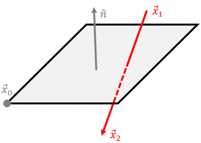
Determine if a line segment intersects a plane is quite easy. A plane is defined as the collection of points \(\vec{x}\) for which
$$\hat{n}\cdot(\vec{x}-\vec{x}_0)=0$$
holds. Here \(\hat{n}\) is the plane normal vector and \(\vec{x}_0\) is some reference point on the plane (otherwise we would have infinitely many parallel planes). We can then simply substitute our definition of the intersection point for \(\vec{x}\) to obtain
$$\hat{n}\cdot\left[\vec{x}_1 + t \left(\vec{x}_2 – \vec{x}_1\right)-\vec{x}_0\right]=0$$
After a bit of algebra, we obtain
$$ t = \frac{\hat{n}\cdot\left(\vec{x}_0-\vec{x}_1\right)} {\hat{n}\cdot\left(\vec{x}_2-\vec{x}_1\right)}, \qquad t\in[0,1]$$
This expression computes the parametric position for the intersectin beween a line and a plane. In order to limit the computation to the segment given by the particle push, we require \(t\in[0,1]\). The data needed for this computation is shown in Figure 2.
Normal Vectors
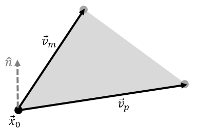
The reference point \(\vec{x}_0\) just needs to be any point known to be on the plane of the triangle. Any of the three vertices will do. In our code we set this to vertex 0 (assuming 0,1,2 numbering). Now what about the normal vector? This is also simple to compute. We use the right hand rule in which we use the right hand to wrap around the triangle in direction 0,1,2. The thumb then gives the direction of the normal vector. Mathematically, we construct a “plus” and “minus” vectors from a vertex, given by
$$\vec{v}_{p,i} = \vec{V}_{i+1}-\vec{V}_{i}$$
and
$$\vec{v}_{m,i} = \vec{V}_{i-1}-\vec{V}_{i}$$
Here \(V_i\) is the position of i-th vertex. We use circular indexing here, so that on \(i=-1\to 2\). The normal vector is then given by
$$\hat{n} = \text{unit}\left(\vec{v}_p \times \vec{v}_m\right)$$
Point in Triangle Check
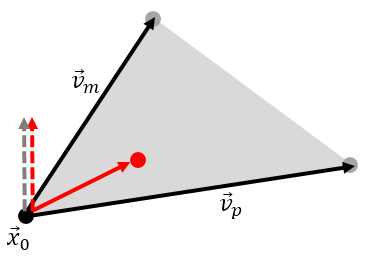
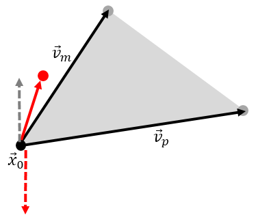
Value \(t\in[0,1]\) from the plane intersection check implies that the line segment intersects the plane of the element. The intersection point could however be outside the bounds of the triangle. We next need to perform a point in triangle test. We first evaluate the actual position of \(\vec{x}_p\) and then use some algorithm to determine if the point is inside or not. Turns out, there are quite a few methods that can be used here. Part of the reason why I wrote this sample code was to give me a simplified environment to test the different algorithms. Running a particle-based code through a profiler, you may find out that some 70% of the total computational time is spent performing these line-triangle intersection tests. Hence, it is important to find an algorithm that not only works, but is also fast. The demo code implements a method based on normal vectors inspired by blackpawn.com. We again compute a normal vector from \(\vec{n}_2=\vec{v}_p \times \vec{v}_m\). However, now instead of \(\vec{v}_p\) being a vector from the vertex to a neighbor vertex, we let it be a vector from the vertex to the intersection point. As long as the intersection point \(\vec{x}_p\) is to the right of the edge vector \(\vec{v}_m\), the computed normal will be parallel with the original triangle normal, \(\vec{n}_2\cdot\hat{n}>0\). This is shown in the first plot in Figure 4. We repeat this algorithm for all three vertices. If the point is outside the triangle, then for at least one vertex, we will have a situation depicted in the second plot of this figure. The intersection point is now to the left of the edge vector \(\vec{v}_m\) and the two normals are anti-parallel, \(\vec{n}_2\cdot\hat{n}<0\). We abort the test once we find such a case as there is no need to check the remaining vertices.
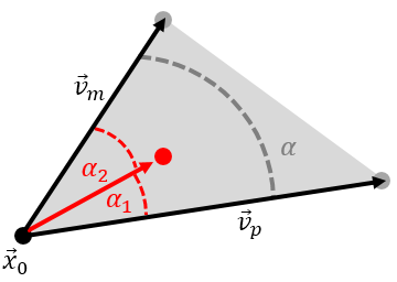
There are many other ways we could use here. Historically, one method I have used a lot is based on angles. Again we loop through all vertixes and on each we generate a vector to the intersection point, \(\vec{v}\). We then compute the angles (or the angle cosines) between this vector and the the two edges. For the point to be in triangle we require \(\alpha_1\le\alpha\) and \(\alpha_2\le\alpha\) on all vertices. Some other methods include computing the areas of the three sub-triangles given by \(\left(\vec{V}_1,\vec{V}_2,\vec{x}_p\right)\), \(\left(\vec{V}_2,\vec{V}_0,\vec{x}_p\right)\), and \(\left(\vec{V}_0,\vec{V}_1,\vec{x}_p\right)\). For the point to be in the triangle we require \(A_0+A_1+A_2=A\), or alternatively
$$T_i = \frac{A_i}{A}\in [0,1] \quad i\in[0,2]$$
where \(T_{i}\) are the three triangle basis functions. We can compute triangle area from
$$A_0 = \frac{1}{2} \left(\vec{x}_p-\vec{V}_1\right) \times \left(\vec{x}_p-\vec{V}_2\right)$$
Off-nominal cases
While the above algorithm is mathematically sound, if you were to implement it as is, you would quickly find that it fails to detect some particle hits. Given the hundreds of millions of surface hits in a typical simulation, it’s inevitable that some particle lands “just right” for the test to fail. The particle then flies out of the computational domain, having “leaked” through a solid boundary. Much of my past time has been spent trying to reduce these leaks but unfortunately I still don’t have a bulletproof solution.
Edge Hits
One of these off-nominal cases is a particle hitting the edge of a triangle. Computer math is not exact and the round off errors mean that we typically need to add a bit of tolerance to account for edge hits. This tolerence effectively grows the triangle, which is also not ideal. Part of the development art is in deciding just how much tolerance to add. Another thing I found to be effective is to use multiple methods to test for a point in triangle. This is in fact what the example code does. It first tests for the point using the method based on normal vectors, but if the point is not inside, it then also tests using the angles based method. The point lies inside as long as either method succeeds. An additional layer could involve recomputing the intersection point using the unique normal vector computed using that vertex edges. The three normals should be the same but computer arithmetic can introduce just enough error to make some edge hits become unacccounted for.
bool SurfaceElement::containsPoint(double p[3], bool primary)
{
	double eps = 1e-4;
	bool check1 = isPointInTriNormals(p,primary,eps);
	bool check2 = false;

	if (!check1) check2 = isPointInTriAngle(p,primary,eps);

	return check1 || check2;
}
Corner Hit
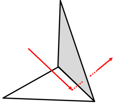
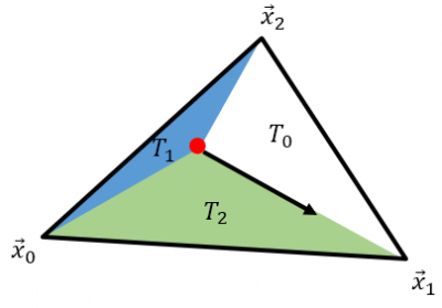
Another difficulty arises with corner hits. In order to avoid self-intersection with the starting surface (after a bounce off), we want the parametric intersection \(t\ge\epsilon_{tol}\), where \(\epsilon_{tol}\) is some small tolerance. This effectively means that we ignore any surface hits that happen within \(t\in[0,\epsilon_{tol})\). This may seem like a non-issue, but given the millions of surface hits, this gap can lead to leaks if a particle happens to land really close to a sharp corner as depicted in Figure 6. I again experimented with several methods to avoid these corner leaks, including using \(\epsilon_{tol}=0\) and flagging and ignoring the surface element from which the particle is rebounding. This unfortunately led to another issue in which a particle would land one an edge shared by multiple elements and then flagging just a single element resulted in the particle becoming stuck to the surface, unable to leave. My current workaround, which is implemented in the example, is to nudge particles landing near edges slightly into the element. This is handled by the SurfaceElement::pushOffEdge method. It uses the triangle basis functions to determine if the particle is on an edge. This approach is not yet optimized as the basis functions could be used to test for the particle in triangle in the first place. If the point is near an edge, it is moved slightly in the direction towards the opposite vertex as also shown in Figure 6.
Overlapping Elements
Ideally we don’t want our mesh containing overlapping elements, but this is not always going to possible. As noted below, I still don’t have a good solution for these.
Quads
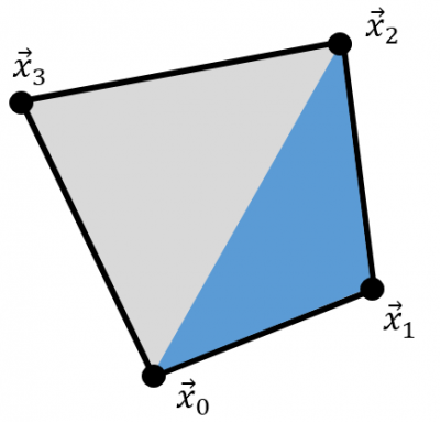
Finally, so far we only discussed triangles. Many of the above methods for testing for a point in triangle could also be used on quads. There is however one major issue: warp. As noted in the introduction, quadrangles produced by common meshing packages will often be non-planar. Therefore, it is much better to internally treat quads as two triangles. We can decompose a quad with vertices (0,1,2,3) into two triangles (0,1,2) and (0,2,3) as shown in Figure 7. This is exactly what the code does. On all surface elements with 4 nodes, the code also computes a secondary normal for the (0,2,3) triangle. Then, when a particle hits a quad, we first perform the line-triangle intersection with the primary (0,1,2) triangle. If intersection is not found, we then next check for a possible intersection against the (0,2,3) triangle. This requires computing a new line-plane intersection point as the two normal vectors may not be identical. Since the post-impact algorithm also needs to know which sub-triangle the particle hit in order to use the correct tangent vectors for the diffuse reflection, we communicate that a secondary triangle was hit by returning
$$t\in[2,3]$$
This is why the particle checking algorithm contains
//obtain parametric position of the intersection point
double t = el->lineIntersect(x_old,part.pos,t_min);

//check for intersection with secondary triangle on warped quads
bool secondary=false;
if (t>=2.0) {t-=2.0;secondary=true;}
Example
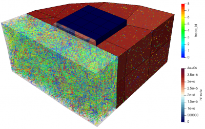
We now have all the pieces to run the code. On Linux, you can compile it with g++ -std=c++11 *.cpp -o surf-int. The simulation generates 100 random particles on the top “source” surface and let’s them bounce over 50,000 time steps. It then saves the surface mesh and several particle traces in a Paraview-compatible format. The surface mesh contains the number of particle hits on each element, scaled by the element area (otherwise larger elements would show more hits). This data and the particle trace is visualized in Figure 8.
Particle Leaks
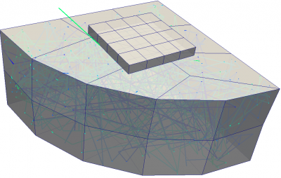
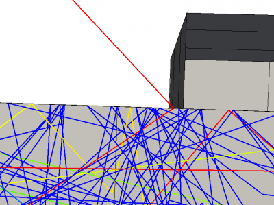
To test for particle leaks, any particle leaving the bounding box of the surface mesh gets removed. If everything went well, we would end the simulation with 100 particles. That is not the case and instead the code finishes with 99 or 98 particles. This translates roughly to a probability of one particle leak per 54,000 surface hits – not exactly ideal. We can add the particle id to the list of traced particles on line 133 to see what exactly is happening. This is shown in Figure 9. The particle hits just below the edge of the overlapping box placed on top of the source. As it rebounds, the code incorrectly thinks the particle is intersecting the vertical face of the box. This error likely arises from the small tolerances added to the point in triangle test. The algorithm that checks for edge impacts pulls the particle upward (into the element). The particle bounces off in diffuse direction computed off this vertical face and escapes our closed volume.
Attachments
Source code: surf-int.zip