Exporting Magnetic Field from FEMM

There is a whole subset of plasma problems that involve non-zero but constant magnetic fields. Ampere’s law tells us that current passing through some medium will induce a magnetic field. However, often these self-induced fields are small enough to be safely neglected. This is especially true if an external magnetic field is applied as is the came with many types of electric propulsion devices. For instance, Hall thrusters and some vacuum arc jets utilize permanent or electromagnets to create a region of relatively strong magnetic field. The strength of this field is several orders of magnitude higher than that of the self-induced fields. We can then assume that \(\partial B/\partial t = 0\), giving us a magnetostatics problem.

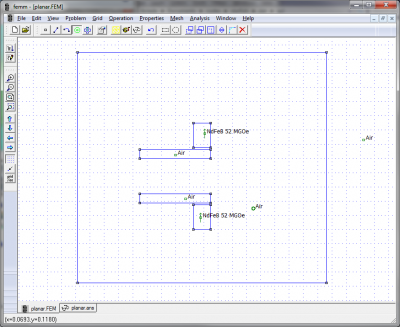
In order to simulate such a problem, we need to know the magnetic field profile. Some codes include a built-in magnetic solver but many others don’t. Such as is the case (at least for now!) with our Starfish code. Starfish requires the magnetic field to be loaded from an input file. Luckily, it is quite easy to model magnetic fields with the FEMM (Finite Element Method Magnetics) program written by David Meeker. FEMM includes a GUI that is used to define the problem geometry, assign material properties, and define boundaries. With a click of a button, the computational mesh is generated and the problem is solved. The code contains a built-in post-processor to view the results.
And here lies the problem with FEMM. While the entire simulation is easily driven from the GUI, the GUI lacks one significant capability: the ability to export 2D results in some standard format for post-processing in a different package! The GUI allows you to only define a line connecting control points and export the data along the line. Doing this for the entire domain would be rather tedious, but it is in fact what we used to do before.
However, some Googling led me to an example code that I have since modified that allows you to export the results automatically by utilizing the built-in Lua scripting language. The code is listed below.
--bf_output.lua--
x1=-0.04
x2=0.04
dx=0.001

y1=0.02
y2=0.06
dy=0.001

ni = (x2-x1)/dx+2
nj = (y2-y1)/dy+2

handle=openfile("B.dat","w")
write(handle,"VARIABLES = x y B Bx Byn")
write(handle,format("ZONE I=%d J=%dn",ni,nj))

for j=0,nj-1,1 do
  for i=0,ni-1,1 do
  x=x1+i*dx
  y=y1+j*dy
  A,B1,B2=mo_getpointvalues(x,y)
  write(handle,x," ",y," ",sqrt(B1*B1+B2*B2)," ",B1," ",B2,"n")
 end
end

closefile(handle)
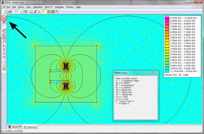
You will want to modify the code based on your domain geometry and the desired output format. This particular incarnation outputs the data in a simple Tecplot format as a rectilinear mesh between (-0.04,0.02) and (0.04,0.06) with uniform mesh spacing of 0.001. To run the script, save the file in the folder with your FEMM input file. Then click the “Open a LUA script” button on top of the toolbar. See Figure 2 below. Select the file and click open. You will only see a message box if something went wrong. On the other hand, if you get no messages, the script ran fine, and you should have a file in your directory named B.dat containing the simulation results. Here we output only the magnetic field vectors and magnitude. You can get additional data from mo_getpointvalues. These are summarized in the reference manual.

It was very helpful. Thanks :).
Very clear, very helpful. Thank you!
Thanks Chris. By the way, I am also a Hokie – I got my B.S. and M.S. from VT, aerospace engineering department.
Thanks so much, this was just the helping hand I needed. In case someone wants to save in a CSV array format, here’s a slight modification.
handlex=openfile(“Bx.csv”,”w”)
handley=openfile(“By.csv”,”w”)
–write(handle,”VARIABLES = x y Bx By\n”)
–write(handle,format(“ZONE I=%d J=%d\n”,ni,nj))
for j=0,nj-1,1 do
for i=0,ni-1,1 do
x=x1+i*dx
y=y1+j*dy
A,B1,B2=mo_getpointvalues(x,y)
write(handlex,B1,”, “)
write(handley,B2,”, “)
end
write(handlex,”\n”)
write(handley,”\n”)
end
closefile(handlex)
closefile(handley)
Then to view in Matlab:
Bx=load(‘Bx.csv’);
figure(1)
hold off;
surf(Bx)
VIEW(2)
Susan,
Your modified code does not work.
Thanks, it is very useful tip.
Thanks a lot! Exactly what I was looking for!
Thank you for this code. It was very helpful. Took some reading to get the code to dump out what I needed from the E field data.
For those who are interested, the following script is based on the above, but tests for “nil” data and produces a txt file with 5 columns. Adjust the spacial range to match your geometry. Combine this with the manual commands and you can get just about any data.
x1=0.0
x2=1.3
dx=0.1
y1=0.0
y2=18.6
dy=0.1
ni = (x2-x1)/dx+2
nj = (y2-y1)/dy+2
handle=openfile(“data.txt”,”w”)
write(handle,”x y V Ex Ey\n”)
for j=0,nj-1,1 do
for i=0,ni-1,1 do
x=x1+i*dx
y=y1+j*dy
V,Ex,Ey=eo_getpointvalues(x,y)
if V ~= nil then
write(handle,x,” “,y,” “,V,” “,Ex,” “,Ey,”\n”)
end
end
end
closefile(handle)
HI
please I dom’t understand X1, x2, y2……dx,dy ?
This is just the Cartesian mesh on which you want to export the data. It’s up to you to decide what you need. (x1,y1) and (x2,y2) are the two diagonal corners and (dx,dy) is the distance between nodes in the x and y direction.
Hi,
I don’t know if I am years too late to get an answer here, but I have basically the same problem.
I have a certain geometry of coils which, through inductive coupling, transform the magnetic field in a given field of interest.
My problem is now, that I want to do post-processing in Origin 9 on the magnetic field data FEMM siumlated. How should I change the Lua code to be able to export an matrix in which I have B-field values for the whole set-up?
Apparently I can also do it manually by defining parallel lines in regular intervalls, but that takes forever.
Every help would be appreciated.
Hi Thomas, if I am understanding your question correctly, you just need to change the x1/x2/y1/y2 points and dx,dy spacing according to your design.
Hi,
I would like to know whether we get only Bx and By from FEMM ? what should we do if we want azimuthal and radial component of the magnetic field obtained.
I think FEMM is only 2D/axisymmetric solver. I need to think about this a bit more but I don’t think that having an azimuthal component makes sense in axisymmetric runs. Such a field would imply that a charged particle has different velocities based on its azimuthal position (specifically based on how much theta it has traversed). But in axisymmetric cases, we assume that there is no variation with theta; all r-z slices are identical.
Here’s a version for an axisymmetric case, with csv output:
r1=1
r2=15
dr=1
z1=-12
z2=12
dz=1
ni = (r2-r1)/dr+2
nj = (z2-z1)/dz+2
handle=openfile(“B.csv”,”w”)
write(handle,”r”,”,”,”z”,”,”,”B”,”,”,”Br”,”,”,”Bz”,”\n”)
for j=0,nj-1,1 do
for i=0,ni-1,1 do
r=r1+i*dr
z=z1+j*dz
A,B1,B2=mo_getpointvalues(r,z)
write(handle,r,”,”,z,”,”,sqrt(B1*B1+B2*B2),”,”,B1,”,”,B2,”\n”)
end
end
closefile(handle)
Hello, could anybody post an example where the (r,z) coordinates are read from an input file? Thank you!
Hi, I’m looking to export a field from an actual setup I’ve simulated so that I can produce some theoretical data in python to go along with the experimental data I already have. How should I change the code to do this and what would be the best format to export the data? Thanks, any help appreciated.