Advection Diffusion Crank Nicolson Solver

Advection Diffusion Equation

Our main focus at PIC-C is on particle methods, however, sometimes the fluid approach is more applicable. One equation that is encountered frequently in the fields of fluid dynamics as well as heat transfer is the advection-diffusion equation. Diffusion is the natural smoothening of non-uniformities. Advection is the motion due to a background flow field. Imagine you drop a cup of coffee into a lake. The initially small, highly concentrated spot will quickly increase in size and the concentration will drop. After some time, the coffee concentration will be roughly uniform. This is diffusion. Now, if the water was moving (as in a river), the coffee blob would start moving along with the stream. This is advection. The combination of these two processes, which is simply a form of mass conservation, reads
$$ \displaystyle \frac{\partial c}{\partial t}+\nabla\cdot\left(-D\nabla c + \vec{u}c\right) = R $$

Below you will find an online solver of this equation. This small CFD program runs completely in your browser and uses Javascript and HTML5 technologies to perform the computations and plotting. The discretization was derived with the Crank Nicolson scheme with the Finite Volume Method and no-flux boundaries.

Online Solver

Click anywhere in the computational space (initially blue box) to start the simulation.

What you should see

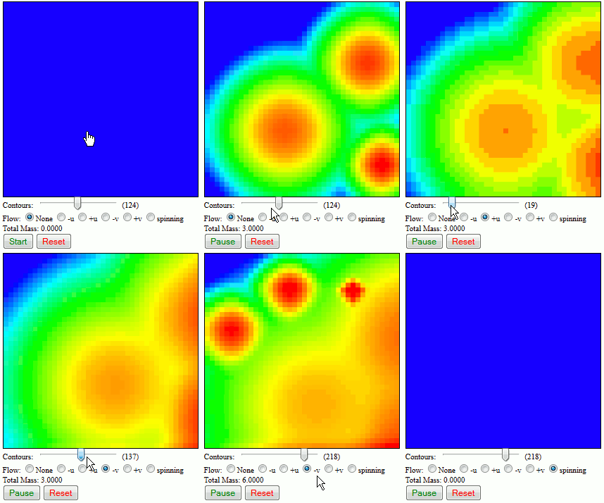
Just in case the demo doesn’t work, the animated .gif below shows you what you should see. Click the mouse to add new sources. You can also use the radio buttons to control the flow field and the number of color levels. Since the code implements zero-flux boundaries, the total mass should remain constant. These boundaries physically correspond to a system where the species is enclosed inside a filter mesh that it cannot penetrate, however, the mesh is permeable to the background flow field. You will see that if you run the code with any of the 4 unidirectional flow fields, all mass will eventually concentrate along a wall. This steady state corresponds to diffusive and advective fluxes balancing each other. The flow carries additional mass towards the wall, but the density gradient limits how much more mass can be deposited. Once the flow is reversed or removed, the concentration will quickly drop.

Finite Volume Formulation

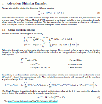
The derivation of the discretized equations for the Finite Volume Method was bit too long to include here as an inline text. Instead, it’s included as a separate pdf:

As mentioned in the notes, this code uses the Crank Nicolson Method to integrate the time derivative. Solving the A-D equation requires marching the solution forward in time. On approach is to use only the data known at current time step to move to the next one. This method, known as as Forward Euler, is the simplest to implement, but it suffers from numerical stability issues. Another method, known as Backward Euler, uses data at the future time step. This is an example of an implicit method, which requires a matrix solution. The Crank Nicolson method combines the two approaches. It is more accurate than the backward Euler since it uses a larger stencil (the collection of nodes used in calculation of each new value).

Javascript + HTML5 CFD Solver

You can download the entire source code here: advection_diffusion.html. The snippet below is the “meat” of the solver. This is the code that builds the matrices and calls the matrix solver.

for (var j=0;j<nj;j++)
	for (var i=0;i<ni;i++)
	{
		var u = t.iju(i,j);
 
		/*reset*/
		a0[u] = 1;	
		a1[u] = 0;
		a2[u] = 0;
		a3[u] = 0;
		a4[u] = 0;
 
		/*RHS*/
		b[u] = 1;
 
		var b0=1;
		var b1=0;
		var b2=0;
		var b3=0;
		var b4=0;
 
		/*east*/
		if (i<ni-1)
		{
			a0[u] += alpha_x  + beta_x*u2[i][j];
			a2[u] += -alpha_x + beta_x*u2[i+1][j];
 
			b0 += -alpha_x - beta_x*u1[i][j];
			b2 += alpha_x - beta_x*u1[i+1][j];
		}
 
		/*west*/
		if (i>0)
		{
			a0[u] += alpha_x - beta_x*u2[i][j];
			a1[u] += -alpha_x - beta_x*u2[i-1][j];
 
			b0 += -alpha_x + beta_x*u1[i][j];
			b1 += alpha_x + beta_x*u1[i-1][j];
		}
 
		/*north*/
		if (j<nj-1)
		{
			a0[u] += alpha_y + beta_y*v2[i][j];
			a4[u] += -alpha_y + beta_y*v2[i][j+1];
 
			b0 += -alpha_y - beta_y*v1[i][j];
			b4 += alpha_y - beta_y*v1[i][j+1];
		}
 
		/*south*/
		if (j>0)
		{
			a0[u] += alpha_y - beta_y*v2[i][j];
			a3[u] += -alpha_y - beta_y*v2[i][j-1];
 
			b0 += -alpha_y + beta_y*v1[i][j];
			b3 += alpha_y + beta_y*v1[i][j-1];
		}
 
		b[u] = b0*t.mesh.c[i][j]+
			   (b1!=0?b1*t.mesh.c[i-1][j]:0) + 
			   (b2!=0?b2*t.mesh.c[i+1][j]:0) +
			   (b3!=0?b3*t.mesh.c[i][j-1]:0) + 
			   (b4!=0?b4*t.mesh.c[i][j+1]:0);
 
		/*add source*/
		b[u] += gamma*(R2[i][j]+R1[i][j]);	
	}
 
/*wrap c*/
var c = t.wrap(t.mesh.c);
 
/*call solver*/
t.solveGS(c,b,a0,a1,a2,a3,a4);
 
/*unwrap*/
t.mesh.c = t.unwrap(c);

The derivation given by the pdf above utilizes velocity and source terms at both current and the future time steps. To simplify the code, these two are assumed to be the same. In other words, fluxes at the k+1 step are computed with the velocities at step k. Same is true for the source term.

Mouse Click Listener

We update the source term on a mouse click (which also seems to work with mobile devices),

function clickListener(e)
{
	/*computes click location*/
	....
 
        /*add source*/
	adcn.mesh.R[i][j] += 1.0/(adcn.mesh.dx*adcn.mesh.dy*adcn.gamma*2);
 
	/*activate button if not running*/
	if (!running) buttonPress();	
}

This term is then cleared at the completion of the time step.

Log Contour Plot

Plotting is performed using the method described in the earlier article on 2D data plotting with HTML5. I don’t yet have a contouring algorithm, so each computational cell is simply flooded according to the cell value, using the rainbow colormap. One difference is that log10 scale is used for the contours. To plot data on a log scale, you simply take log of all parts of the interpolation equation. We have

var log_min = log10(1e-3);
var log_max = log10(1e4);
...	
var z = (log10(data[i][j]) - log_min)/(log_max-log_min);

where I used (although didn’t have to, since the denominator cancels out…)

function log10(a) {return Math.log(a)/Math.LOG10E;}

The time stepping is performed using window.requestAnimationFrame. This is the new preferred way over setTimeout. The code that would normally reside in the main for loop of a stand-alone solver is placed into a callback that is repeatedly called using this method. The code is below

p.timeStep = function()
{
	if (spinning)
	{
        /*code to rotate velocity field*/
	}
 
	t.marchADCN();
	if ((t.it++)%5==0) replot();
 
	if (running)
		window.requestAnimationFrame(t.timeStep);
}

Closing Notes

HTML5 introduces web workers for creation of tasks that run in background. Using workers would be probably necessary in order to generate a more detailed solver. I didn’t use them in this case, partly to keep things simple, and partly because I wasn’t sure how efficient this method would be given the large amount of data transfer needed to make animation plots. But at any rate, there is a great overview of workers at html5rocks.com.

Finally, don’t hesitate to leave a comment if something is not clear.